Graptolite Synonymies
Correlation to temporal, geographic, or authorial factors?
Erin Schuster
Introduction
Taxonomy is the method by which organisms are assigned to a genus and species group. It is a science that is constantly evolving due to our growing knowledge of a group of organisms. This is especially true of graptolite taxonomy. Early work with graptolites focused solely on naming graptolites for use in biostratigraphy, meaning that graptolites were loosely grouped based on their general appearance instead of evolutionary or trait based backing. As studies into the evolution in graptolite morphology, or genetics based traits increased, there was an increasing realization that synonymies, or the same type of organism with different taxonomic names, existed. Through carefully examination of graptolite literature these synonyms are slowly being identified (Mitchell et al., unpublished data). However, the presence of synonyms may not only be due to changes in graptolite research through time. These synonyms may be geographically located either due to a cultural preference for generating new species or a tectonically strained region where morphology is more difficult to constrain. It may also be that particular authors were more likely to generate new species names due to a variety of factors.
This research will attempt to examine any correlation by first mapping the presence of graptolites that both with and without synonyms on a world map to visually determine locations with more synonymies. This map will then be animated such that the graptolite locations will plot based upon the year that they were named. If there is a temporal correlation to synonymies, more synonyms should plot within a given time frame than others. Finally, the graptolites with synonyms will be grouped by the original naming author with the number of individual species summed per author to determine if there is an author based correlation.
Materials and methods
The presence of graptolite synonymies may be correlated to a number of factors including time, cultural or tectonic location, and author. The project will combine data on synonymies, contained within the Taxonomic Dictionary (Mitchell et al., unpublished data), with graptolite locatlity information, complied as section data (Mitchell et al., unpublished data). This will be used to:
1. Examine geographic distribution of graptolites with synonymies compared to graptolites without synonymies
2. Examine temporal distribution of graptolite synonymies
3. Determine the number of synonymies based on naming author
4. Determine number of synonymies per author per year.
Intially, the required packages will need to be loaded (you may need to install some packages):
library(dplyr)
library(tidyr)
library(sp)
library(rgeos)
library(maptools)
library(ggplot2)
library(ggmap)
library(maptools)
library(maps)
library(leaflet)
library(htmlwidgets)
library(widgetframe)
library(DT)
library(devtools)
library(RCurl)
library(httr)
library(gganimate)
The data are contained in two comma separated files (CSV), the Taxonomic Dictionary and the section data.
#Load Taxonomic Dictionary

myDict=read.csv("data/Taxonomic dictionary Oct3'17_mod.csv",header=T,sep=",")

#Load section data

mySect=read.csv("data/sections_table format.csv", header=T, sep =",")
Geographic Methodology
After loading both CSV files, the section data and the Taxonomic Dictionary must be joined so that all the geographic locations are paired with the correct taxonomic information including the presence of senior synonyms. These data are then filtered by the senior synonym column in order to generate a list that contains only graptolite locations with named senior synonyms.
#Join the sections data and the graptolite dictionary
Grap_locate=full_join(mySect,myDict,by="GRCode")

#Generate synonoym list
synGrap_locate=filter(Grap_locate, senior.synonym!="*" & senior.synonym!=99999)
These two data sets are visually compared by overlapping the synonyms list over all of the graptolite locations on a world map.
Grap_map_inter=leaflet() %>%
  addTiles() %>%
  addCircles(data=Grap_locate,group="All Graptolite Locations",color="red") %>%
  addCircles(data=synGrap_locate,group="Graptolite Synonym Locations",color="blue") %>%
  addLayersControl(overlayGroups=c("All Graptolite Locations","Graptolite Synonym Locations"), options=layersControlOptions(collapsed=F))
frameWidget(Grap_map_inter,height = 500)
The synonymies are then filtered by the decade in which they were named, beginning in 1828 with the first named species.
# Filter by "decade"
synGrap_year=filter(synGrap_locate, date!="*" & date!="Chen et al 2011" & date!="1997a")

synGrap_18_2837=filter(synGrap_year, date==1828 | date==1829 | date==1830 | date==1831 | date==1832 | date==1833 | date==1834 | date==1835 | date==1836 | date==1837)
synGrap_18_3847=filter(synGrap_year, date==1838 | date==1839 | date==1840 | date==1841 | date==1842 | date==1843 | date==1844 | date==1845 | date==1846 | date==1847)
synGrap_18_4857=filter(synGrap_year, date==1848 | date==1849 | date==1850 | date==1851 | date==1852 | date==1853 | date==1854 | date==1855 | date==1856 | date==1857)
synGrap_18_5867=filter(synGrap_year, date==1858 | date==1859 | date==1860 | date==1861 | date==1862 | date==1863 | date==1864 | date==1865 | date==1866 | date==1867)
synGrap_18_6877=filter(synGrap_year, date==1868 | date==1869 | date==1870 | date==1871 | date==1872 | date==1873 | date==1874 | date==1875 | date==1876 | date==1877)
synGrap_18_7887=filter(synGrap_year, date==1878 | date==1879 | date==1880 | date==1881 | date==1882 | date==1883 | date==1884 | date==1885 | date==1886 | date==1887)
synGrap_18_8897=filter(synGrap_year, date==1888 | date==1889 | date==1890 | date==1891 | date==1892 | date==1893 | date==1894 | date==1895 | date==1896 | date==1897)
synGrap_1819_9807=filter(synGrap_year, date==1898 | date==1899 | date==1900 | date==1901 | date==1902 | date==1903 | date==1904 | date==1905 | date==1906 | date==1907)
synGrap_19_0817=filter(synGrap_year, date==1908 | date==1909 | date==1910 | date==1911 | date==1912 | date==1913 | date==1914 | date==1915 | date==1916 | date==1917)
synGrap_19_1827=filter(synGrap_year, date==1918 | date==1919 | date==1920 | date==1921 | date==1922 | date==1923 | date==1924 | date==1925 | date==1926 | date==1927)
synGrap_19_2837=filter(synGrap_year, date==1928 | date==1929 | date==1930 | date==1931 | date==1932 | date==1933 | date==1934 | date==1935 | date==1936 | date==1937)
synGrap_19_3847=filter(synGrap_year, date==1938 | date==1939 | date==1940 | date==1941 | date==1942 | date==1943 | date==1944 | date==1945 | date==1946 | date==1947)
synGrap_19_4857=filter(synGrap_year, date==1948 | date==1949 | date==1950 | date==1951 | date==1952 | date==1953 | date==1954 | date==1955 | date==1956 | date==1957)
synGrap_19_5867=filter(synGrap_year, date==1958 | date==1959 | date==1960 | date==1961 | date==1962 | date==1963 | date==1964 | date==1965 | date==1966 | date==1967)
synGrap_19_6877=filter(synGrap_year, date==1968 | date==1969 | date==1970 | date==1971 | date==1972 | date==1973 | date==1974 | date==1975 | date==1976 | date==1977)
synGrap_19_7887=filter(synGrap_year, date==1978 | date==1979 | date==1980 | date==1981 | date==1982 | date==1983 | date==1984 | date==1985 | date==1986 | date==1987)
synGrap_19_8897=filter(synGrap_year, date==1988 | date==1989 | date==1990 | date==1991 | date==1992 | date==1993 | date==1994 | date==1995 | date==1996 | date==1997)
synGrap_1920_9807=filter(synGrap_year, date==1998 | date==1999 | date==2000 | date==2001 | date==2002 | date==2003 | date==2004 | date==2005 | date==2006 | date==2007)
synGrap_20_0817=filter(synGrap_year, date==2008 | date==2009 | date==2010 | date==2011 | date==2012 | date==2013 | date==2014 | date==2015 | date==2016 | date==2017)
These subdivisions are mapped on a world map as individual layers to indicate any geographic relation in the above decadal time breaks.
Grap_decade_inter=leaflet() %>%
  addTiles() %>%
  addCircles(data=Grap_locate,group="All Graptolite Locations",color="red") %>%
  addCircles(data=synGrap_18_2837,group="Graptolite Synonymies 1828-1837",color="blue") %>%
  addCircles(data=synGrap_18_3847,group="Graptolite Synonymies 1838-1847",color="blue") %>%
  addCircles(data=synGrap_18_4857,group="Graptolite Synonymies 1848-1857",color="blue") %>%
  addCircles(data=synGrap_18_5867,group="Graptolite Synonymies 1858-1867",color="blue") %>%
  addCircles(data=synGrap_18_6877,group="Graptolite Synonymies 1868-1877",color="blue") %>%
  addCircles(data=synGrap_18_7887,group="Graptolite Synonymies 1878-1887",color="blue") %>%
  addCircles(data=synGrap_18_8897,group="Graptolite Synonymies 1888-1897",color="blue") %>%
  addCircles(data=synGrap_1819_9807,group="Graptolite Synonymies 1898-1907",color="blue") %>%
  addCircles(data=synGrap_19_0817,group="Graptolite Synonymies 1908-1917",color="blue") %>%
  addCircles(data=synGrap_19_1827,group="Graptolite Synonymies 1918-1927",color="blue") %>%
  addCircles(data=synGrap_19_2837,group="Graptolite Synonymies 1928-1937",color="blue") %>%
  addCircles(data=synGrap_19_3847,group="Graptolite Synonymies 1938-1947",color="blue") %>%
  addCircles(data=synGrap_19_4857,group="Graptolite Synonymies 1948-1957",color="blue") %>%
  addCircles(data=synGrap_19_5867,group="Graptolite Synonymies 1958-1967",color="blue") %>%
  addCircles(data=synGrap_19_6877,group="Graptolite Synonymies 1968-1977",color="blue") %>%
  addCircles(data=synGrap_19_7887,group="Graptolite Synonymies 1978-1987",color="blue") %>%
  addCircles(data=synGrap_19_8897,group="Graptolite Synonymies 1988-1997",color="blue") %>%
  addCircles(data=synGrap_1920_9807,group="Graptolite Synonymies 1998-2007",color="blue") %>%
  addCircles(data=synGrap_20_0817,group="Graptolite Synonymies 2008-2011",color="blue") %>%
  addLayersControl(overlayGroups=c("All Graptolite Locations","Graptolite Synonymies 1828-1837","Graptolite Synonymies 1838-1847",
                                   "Graptolite Synonymies 1848-1857","Graptolite Synonymies 1858-1867","Graptolite Synonymies 1868-1877",
                                   "Graptolite Synonymies 1878-1887","Graptolite Synonymies 1888-1897","Graptolite Synonymies 1898-1907",
                                   "Graptolite Synonymies 1908-1917","Graptolite Synonymies 1918-1927","Graptolite Synonymies 1928-1937",
                                   "Graptolite Synonymies 1938-1947","Graptolite Synonymies 1948-1957","Graptolite Synonymies 1958-1967",
                                   "Graptolite Synonymies 1968-1977","Graptolite Synonymies 1978-1987","Graptolite Synonymies 1988-1997",
                                   "Graptolite Synonymies 1998-2007","Graptolite Synonymies 2008-2011"),
                   options=layersControlOptions(collapsed=F))
frameWidget(Grap_decade_inter,height = 500)
However, there is more variation in the number and locations of synonymies by year that is time averaged on the decade scale. This differentiation is displayed using an animation which displays every year in the dataset.
worldmap=borders("world",colour="gray50",fill="white")
mapWorld=ggplot()+worldmap

Grap_map=
  mapWorld+
  geom_point(data=Grap_locate,aes(x=Longitude,y=Latitude),col="red")+
  geom_point(data=synGrap_locate,aes(x=Longitude,y=Latitude,frame=date),col="blue")+
  coord_equal()

gganimate(Grap_map,interval=3.5)
#interval is in secondsResults
As research into graptolite taxonomy has developed and grown, graptolite names and naming procedures have also evolved. As a result, many graptolites that were originally named for biostratigraphy or in the earliest periods of graptolite research have synonymies. These synonymies were analyzed to determine if there was a correlation to their geography, when the graptolites were named, or who the naming authors were.
Due to the nature of graptolite preservation and collection, no geographical analysis of synonym locations would yield any illuminating results. Any analysis shows that the graptolites are highly clustered. However, figure 1 clearly shows that the majority of the locations where graptolites have been collected are locations where synonymies occur. This is most likely due to the nature of the graptolite Taxonomic Dictionary. The Taxonomic Dictionary mostly contains graptolites which occur globally as these are more useful to wider research applications than endemic or local species. As such, the distribution of synonyms may vary as more endemic species are added to the Dictionary.Figure 1. Map illustrating locations of graptolites and graptolite synonymies. All graptolite locations are red and locations with graptolite synonymies are blue.
Since there is no correlation strictly between geography and graptolite synonyms, the locations were divided into the decades in which the graptolites were named, starting in 1828 (Figure 2). Again, due to the nature of graptolite collection and preservation, there are no analyses that will show the data as anything other than clustered and having a global distribution.
Figure 2. Map of graptolite locations grouped by decade. All graptolite locations are red and locations with graptolite synonymies are blue.
While the decadal categories show that there are temporal differences in the number of graptolites with synonymies, the majority in these variations are “time averaged” by being grouped together. As such, the animation in figure 3 cycles through every year contained in the data set, starting in 1828. Most notably, there are no graptolite synonymies during the years: 1855-56, 1863, 1878, 1887, 1889, 1892, 1912, 1916-1919, 1922, 1928, 1930, 1940, 1943, 1945-46, 1950, 1957, 1961, 1966, 1985, 1992, 1996, 2002, 2004, and 2007. In addition, there appears to be regional isolation of graptolite synonymies named in the years: 1857, 1882-83, 1891, 1896-97, 1903, 1911, 1913-1915, 1926-27, 1938, 1942, 1944, 1953, 1955-56, 1959, 1968, 1972, 1981, 1990, 1994-95, 1997, 2001, and 2003. These locations may be significant, however further investigation is needed.
Figure 3. Animation of graptolite synonymies per year.
In addition to geography, graptolite synonymies could be correlated to the year the species were named or the naming author. This is analyzed by grouping the graptolite synonymies by year, by author, and by author and year (Tables 1, 2, and 3).
Table 1. Number of graptolites with a synonym per year.
Table 2. Number of graptolites with a synonym per author.
Table 3. Number of graptolites with synonyms per author per year.
Using two chi-squared tests for each potential correlation, grouping by year, by author, and by author and year are all significantly different than a random distribution. However, only the two year and author groupings are significantly different than a uniform, or expected distribution. The author and year grouping has a p-value of 0.966, meaning that it is not significantly different.
Results of chi-square tests of data grouped by year:
##
##  Chi-squared test for given probabilities with simulated p-value
##  (based on 1000 replicates)
##
## data:  synGrap_yearcount$n
## X-squared = 1136.8, df = NA, p-value = 0.000999
##
## Pearson's Chi-squared test
##
## data: rbind(synGrap_year_expct$n, synGrap_year_expct$expected)
## X-squared = 453.41, df = 144, p-value < 2.2e-16Results of chi-square tests of data grouped by author:
##
##  Chi-squared test for given probabilities with simulated p-value
##  (based on 1000 replicates)
##
## data:  synGrap_authorcount$n
## X-squared = 5726.2, df = NA, p-value = 0.000999
##
## Pearson's Chi-squared test
##
## data: rbind(synGrap_author_expect$n, synGrap_author_expect$expected)
## X-squared = 904.17, df = 421, p-value < 2.2e-16Results of chi-squared tests of data grouped by author and year:
##
##  Chi-squared test for given probabilities with simulated p-value
##  (based on 1000 replicates)
##
## data:  synGrap_authoryear$n
## X-squared = 1798.7, df = NA, p-value = 0.000999
##
## Pearson's Chi-squared test
##
## data: rbind(synGrap_authoryear_expect$n, synGrap_authoryear_expect$expected)
## X-squared = 523.43, df = 731, p-value = 1The above analyses raise the question if there is a significant difference between the number of renamed graptolites and the number of senior synonyms when grouped by author and year (Table 4).
Table 4. Number of renamed graptolites versus senior synonyms grouped by author and year.
Results of the chi-squared test of data grouped by author and year:
##
##  Pearson's Chi-squared test with simulated p-value (based on 1000
##  replicates)
##
## data:  Grap_authoryear$`n senior.synonym` and Grap_authoryear$`n renamed`
## X-squared = 1255.1, df = NA, p-value = 0.000999
The chi-squared test has a p-value of 0.000999 indicating a statistical difference between the number of renamed graptolites and senior synonyms when grouped by author and year.
Finally, the cumulative sum of the number of renamed graptolites and senior synonyms are plotted by date (Figure 4).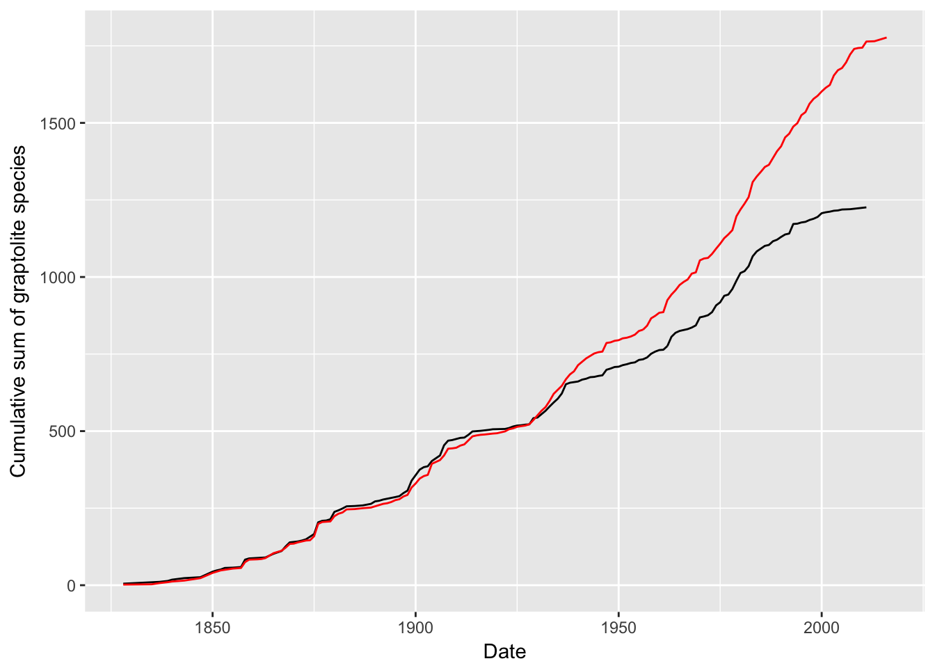
Figure 4. Line graph of the cumulative sum of the number of renamed graptolites (black) versus the number of senior synonyms (red) over time.
The line graph shows that the number of renamed graptolites and the number of senior synonyms follows the same line until about the 1930s. At that point, the two groups begin to diverge, with the number of senior synonyms continuing to grow while the number of renamed graptolites begins to level off in the early 2000s.
Conclusions
As the study of graptolite taxonomy has developed, there have been many changes to graptolite naming procedures and to the names of graptolite species themselves. As a result of this progression, there is a statistically significant temporal correlation with the number of graptolite synonymies, based on the results of the chi-squared analyses of both random and uniform distributions. While this gives the impression of a general decrease in the number of synonymies generated over time, the greatest number of graptolites with synonyms occurred in 1876, 48 years after the first named graptolite in the Taxonomic Dictionary. In fact, the year 1828 has only 5 graptolites with synonyms (Table 1). This indicates that the temporal correlation is not as straight forward as could be presumed.
The next reasonable correlation to the number of graptolite synonymies are the naming authors. Due to either the time period in which the authors were most prolific or due to the author’s general lack of knowledge of graptolites, there is a statistically significant correlation between the number of graptolite synonymies and the naming author as a result of the chi-squared analyses. The pair of authors with the most synonyms are Elles & Wood (Table 2). However, this brings to question whether there is a combined correlation to the number of synonymies and the both the naming author and the year the species was named.
This inquiry shows that while the correlation between the number of graptolite synonymies and author paired with year is significantly different than a random distribution, it is not significantly different than a uniform distribution. Further investigation is needed to determine what the broader implications of this is. However, in 1876 the 38 graptolites with synonyms were either named by or attributed to the author Lapworth and Elles & Wood named 22 graptolite species in 1907 which were later assigned a senior synonym (Table 3). This seems to indicate that while the relationship may not be as strong there is a correlation between the naming author and the year named to the number of graptolite synonymies.
Finally, the number of graptolite synonymies were compared to the number of graptolite senior synonyms when grouped by author and by year. A chi-squared analysis shows that the two categories are statistically different than each other. In addition, the greatest number of senior synonyms were named by Lapworth in 1876 (Table 4). This shows that not all the graptolites named in the early days of graptolite paleontology require renaming as methodologies advance. In addition, the number of renamed graptolites have greatly decreased since the 1930’s and 40’s (Table 4, Figure 4). This progression of decreasing number of graptolites with senior synonyms should continue in the future as more graptolites are named based on modern taxonomic conventions.
Unlike the results above, the number of graptolite synonymies does not seem to have a visual correlation related to geography. This is most likely due to both the global nature of the graptolites contained in the graptolite Taxonomic Dictionary, but also due to the clustered nature of graptolite preservation and collection. Further investigation is needed to determine if there is any significance to graptolite synonymies isolated to particular regions as observed in Figure 3.
References
Mitchell, Charles et al., Graptolite Sections Data, unpublished data.
Mitchell, Charles et al., Graptolite Taxonomic Dictionary, unpublished data.